Categorical Data Analysis

The following statistical indices are output when the categorical data analysis of Exametrika is used.

l Threshold

l Entropy

l Biserial correlation coefficient (polyserial correlation coefficient)

l Tetrachoric correlation coefficient (polychoric correlation coefficient)

Threshold

l Dichotomous (binary) data

First, a standard normal distribution is assumed underlying the data. In such a assumption, when the correct response rate for an item is 0.85, the threshold would be -1.04, as shown in the left-hand side figure. The threshold is obtained when the area above the threshold is equal to the correct response rate. The item on the left-hand side can be interpreted as an item with correct responses by the examinees, whose capability is -1.04 or above within the standard normal distribution. The figure on the right-hand side, on the other hand, represents an item with a correct response rate of 10%. In this case, the threshold becomes 1.28, which is interpreted as an item that cannot have correct responses unless a person has a high ability level of 1.28 or higher within the standard normal distribution.

l Polytomous (categorical ordered) data

If there are K categories, there are K-1 thresholds. Let us assume that there is an item with four ordered categories, when selection rates are 0.2, 0.4, 0.3, and 0.1. In such an instance, the three thresholds are derived by dividing the area of the standard normal distribution to obtain the selection rates described above.

Entropy

Entropy is an index like the variance for categorical data (qualitative data). When every examinee’s choice concentrates on a specific category, entropy approaches 0. The value of entropy increases, however, as the selections of examinees become more dispersed (not concentrated). In general, no information exists for items for which there is a concentration of category choices, as it would be the same whether or not a question was asked. Very small items of entropy are often inappropriate as an item.

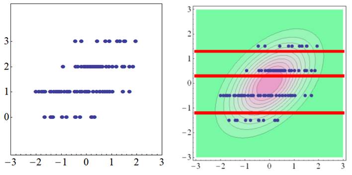
Biserial correlation (polyserial correlation)

l Biserial correlation (dichotomous variable × continuous variable)

A correlation coefficient can be estimated by maximizing the occurrence probability (likelihood) after assuming a 2-variate standard normal distribution behind dichotomous categorically ordered data and continuous data. The correlation coefficient obtained in this manner is called the biserial correlation coefficient.

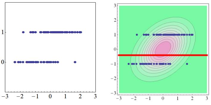
The diagram above indicates a trend, wherein a slight tendency exists for variables of the X-axis to be higher when the dichotomous data of the Y-axis is 1. A 2-variate standard normal distribution with a moderate correlation fits in the background of the 2-variate data in such instances. Furthermore, the threshold (marked with a red line) comes slightly under the peak of the 2-variate normal distribution, since the number of observations is slightly larger when the dichotomous variable of the Y-axis is 1.

The 2-variate normal distribution with a negative correlation fits behind the dichotomous variables since the continuous variables tend to be larger when the variables on the Y-axis are 0 in the diagram above. The biserial correlation coefficient is therefore obtained from the perspective of a 2-variate normal distribution with how size of the correlation fits best with the data. A correlation that is more reasonable than calculating a Pearson correlation by assuming dichotomous data to be continuous is obtained in this way.

l Polyserial correlation (polytomous variable × continuous variable)

The biserial correlation extended to polytomous data is referred to as the polyserial correlation. The Likert scale data often used in psychological questionnaires and social surveys is, in the strict sense, a categorically ordered data with inconsistent intervals. Therefore, the Likert data with very few categories, such as three-point ratings and four-point ratings, are not considered as continuous data but should be treated as categorically ordered data.

Tetrachoric correlation (polychoric correlation)

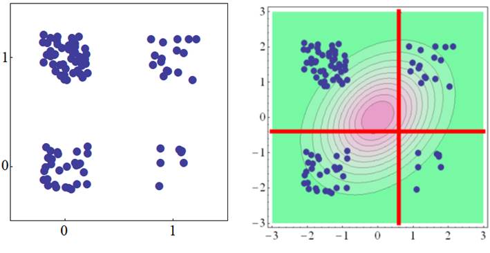
l Tetracoric correlation (dichotomous variable × dichotomous variable)

The scatter plots shown on the top-left and bottom-left panels are of two dichotomous variables. The correlation coefficient that maximizes the occurrence probability (likelihood) by assuming a 2-variate standard normal distribution behind these two variables is called the tetrachoric correlation.

There is more data when the dichotomous variable of the X-axis is 0 in the diagram above, thus the threshold (red vertical line) along the X-axis is positioned in the positive direction from the peak of the 2-variate normal distribution. Furthermore, the threshold of the Y-axis (red horizontal line) is slightly to the negative side of the peak, as there is more data when the dichotomous variable of the Y-axis is 1. Furthermore, of the data that was divided into four, the number of data for (1, 1) and (0, 0) is slightly greater than that for (0, 1) and (1, 0); thus, the tetrachoric correlation is obtained to be positive.

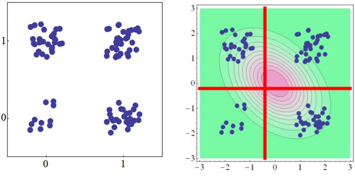
Inversely, this data is more likely to occur when the 2-variate normal distribution with a negative correlation is set behind this data, since in the diagram above the number of data for (1, 0) and (0, 1) is greater than the number of data for (1, 1) and (0, 0). Therefore, in such situations, the tetrachoric correlation is obtained as a negative value.

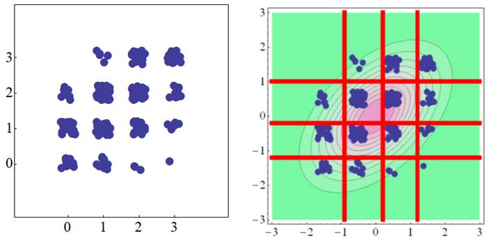
l Polychoric correlation (polytomous variable × polytomous variable)

The polychoric correlation is an extension of the tetrachoric correlation to a correlation between the polytomously categorical variables. Since the Likert scale data, often seen with psychological questionnaires and social surveys, do not have exactly equal intervals. When the number of categories is small, such as with three-point or four-point ratings, a more reasonable correlation is obtained by treating it as categorically ordered data, rather than computing a Pearson correlation coefficient by considering it to be continuous data.